http://cdn.mathjax.org/mathjax/latest/MathJax.js
Motivation
As I am going back to the Philippines to pursue further studies in Statistics, it intrigues me if Data Mining and Data Science are catching up. I am seeing some positions in jobsearch websites such as Jobstreet so as a data miner, I extracted the relevant job openings that are related to the key phrases:
- Data Mining; and
- Data Scientist.
These may look too specific but this is just a quick draft, anyway. Also, I did not include Data Analyst as this scopes a broader job scope diversity than the two mentioned. Also any intensive text extraction using basic Information Retrieval methods is not used.
Warning: The result of the models should not be used to provide recommendations as data the is collected using a convenience sample without performing accuracy tests, only k-fold cross validations against the training set when CART is used.
Data Set
The data is collected manually by searching for relevant job openings active today, 22 May, 2015. I have an assumption that that the data set is relatively small, and so less than 30 positions is returned. Pre-processing is done externally, in Excel, to remove currency prefix, i.e. PHP and text in experience, etc.
library(RCurl)
jobstreet <- getURL("https://raw.githubusercontent.com/foxyreign/Adhocs/master/Jobstreet.csv", ssl.verifypeer=0L, followlocation=1L) # Download from github
writeLines(jobstreet, "Jobstreet.csv")
df <- read.csv('Jobstreet.csv', head=T, sep=",") # Load dataset
df <- na.omit(df) # Exclude missing data

summary(df) # Summarize
## Expected.Salary Experience Education
## Min. : 11000 Min. : 0.000 Min. :1.000
## 1st Qu.: 19000 1st Qu.: 2.000 1st Qu.:2.000
## Median : 28000 Median : 4.000 Median :2.000
## Mean : 35016 Mean : 4.919 Mean :2.179
## 3rd Qu.: 40000 3rd Qu.: 8.000 3rd Qu.:2.000
## Max. :130000 Max. :20.000 Max. :4.000
##
## Specialization Position
## IT-Software :30 Data Mining :72
## - :17 Data Scientist:51
## IT-Network/Sys/DB Admin:14
## Actuarial/Statistics :12
## Banking/Financial : 8
## Electronics : 8
## (Other) :34As mentioned, there are only approximately 120 job applicants which applied for these two grouped positions. Since the data does not mention if an applicant applied for more than one position, I assume that these are distinct records of applicants per position and/or position group, Data Mining and Data Scientist.
Variables
- Expected.Salary – numerical. The expected salary of each applicant based on their profile.
- Experience – ordinal but treated as numerical for easier interpretation in the later algorithms used. This is the years of work experience of the applicant.
- Education – categorical; not used in the models because of extreme unbalance in proportions. This is labelled as:
- 1 – Secondary School
- 2 – Bachelor Degree
- 3 – Post Graduate Diploma
- 4 – Professional Degree
- Specialization – categorical; not used in this analysis.
- Position – categorical. Data Mining or Data Scientist
- Education.Group – categorical. Additional variable to bin the years of experience.
# Categorize education variable
df$Education <- factor(df$Education, levels = c(1,2,3,4),
                       labels=(c("Secondary Sch", "Bach Degree",
                                 "Post Grad Dip", "Prof Degree")))

# Bin years of experience
df$Experience.Group <- ifelse(df$Experience < 3, "3 Years",
                              ifelse(df$Experience < 5, "5 Years",
                                     ifelse(df$Experience < 10, "10 Years", "+10 Years")))
df$Experience.Group <- factor(df$Experience.Group,
                              levels=c("3 Years", "5 Years", "10 Years", "+10 Years"))

# Drop variables
df <- df[, !(colnames(df) %in% c("Education","Specialization"))]

# Subsets positions
mining <- subset(df, Position == "Data Mining")
scientist <- subset(df, Position == "Data Scientist")
Distribution
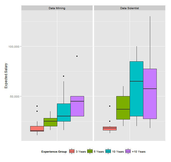
As expected, Data Scientists have a higher expected salary although this is so dispersed that even if I compare these two using a t-test assuming heteroskedastic distribution, there is a significant difference between the averages expected salaries of the two positions.
require(ggplot2)
require(scales)

# Boxplot
ggplot(df, aes(x=factor(0), y=Expected.Salary, fill=Experience.Group)) +
  facet_wrap(~Position) + geom_boxplot() + xlab(NULL) +
  scale_y_continuous(labels = comma) +
  theme(axis.title.x=element_blank(),
        axis.text.x=element_blank(),
        axis.ticks.x=element_blank(),
legend.position="bottom") |
| Distribution of Expected Salaries |
# T-test
t.test(Expected.Salary ~ Position, paired = FALSE, data = df)
##
## Welch Two Sample t-test
##
## data: Expected.Salary by Position
## t = -3.3801, df = 68.611, p-value = 0.001199
## alternative hypothesis: true difference in means is not equal to 0
## 95 percent confidence interval:
## -24086.501 -6205.983
## sample estimates:
## mean in group Data Mining mean in group Data Scientist
## 28736.11 43882.35# Median expected salaries of Data Mining vs Data Scientist
c(median(mining$Expected.Salary), median(scientist$Expected.Salary))## [1] 25000 30000Come on fellow data enthusiasts, you should do better than this! The difference of their medians is just 5,000 PHP. In my honest opinion, these center values are way below based on the prospective demand of shortage of these people who can understand data in the next 10 years.
Regression
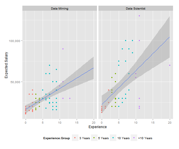
The intercept is not included in the model because I want to see the contrast between Data Mining and Data Scientist although I already computed it beforehand. Besides, though the linear regressio model shows significant value, but when doing diagnostics, linear approach is not appropriate because the residual errors are not random and depict a funnel shape based on their errors. The quantitative measures of regressions for significance cutoff are: $r_{adj}^{2}>0.80, p<0.05$
The regression output coefficients are interpreted as follows:
$$y = \beta_{0}(12,934.9) + \beta_{1}(3,336.3) + \beta_{2}$$
# Estimate coefficients of linear regression model
summary(lm(Expected.Salary ~ Experience + Position-1, data=df))
## Call:
## lm(formula = Expected.Salary ~ Experience + Position - 1, data = df)
##
## Residuals:
## Min 1Q Median 3Q Max
## -45312 -11123 -1280 6877 66688
##
## Coefficients:
## Estimate Std. Error t value Pr(>|t|)
## Experience 3336.3 446.3 7.476 1.38e-11 ***
## PositionData Mining 12934.9 3024.3 4.277 3.83e-05 ***
## PositionData Scientist 26612.0 3455.8 7.701 4.27e-12 ***
## ---
## Signif. codes: 0 '***' 0.001 '**' 0.01 '*' 0.05 '.' 0.1 ' ' 1
##
## Residual standard error: 18350 on 120 degrees of freedom
## Multiple R-squared: 0.8136, Adjusted R-squared: 0.809
## F-statistic: 174.6 on 3 and 120 DF, p-value: < 2.2e-16# Scatter plot
ggplot(df, aes(x=Experience, y=Expected.Salary)) +
geom_point(aes(col=Experience.Group)) +
facet_wrap(~Position) +
scale_y_continuous(labels = comma) +
stat_smooth(method="lm", fullrange = T) +
theme(legend.position="bottom") |
| Scatterplot of Expected Salary per Year of Experience |
# Diagnose LM
par(mfrow=c(1,2))
plot(lm(Expected.Salary ~ Experience + Position-1, data=df), c(1,2)) |
| Linear Regression Estimates and Diagnostics |
CART
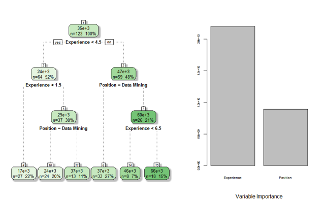
Information Gain is used to divide the nodes based on weighted average entropy as linear regression does not do well with the data set. Of course, years of experience is more influential than the position.
Looking at the estimated salaries from the printed tree, applicants who have years of experience lower than 1.5 are approximately expecting 17,000 PHP. While those who applied for Data Mining jobs with more than 6.5 years of experience are expecting 66,000 PHP on average.
require(rpart)
require(rattle)

cart <- rpart(formula = Expected.Salary ~ Experience + Position,
              data = df,
              parms = list(split = "information"), # Uses information gain
              model = T) # Retains model information

# Plot tree
layout(matrix(c(1,2,3,4), nrow = 1, ncol = 2, byrow = TRUE), widths=c(1.5,2.5))
barplot(cart$variable.importance,
        cex.names = 0.6, cex.axis = 0.5,
        sub = "Variable Importance")
fancyRpartPlot(cart, main=NULL, sub=NULL) |
| Decision Tree using CART and Variable Importance |
# Estimates
print(cart); printcp(cart)
## n= 123
##
## node), split, n, deviance, yval
##       * denotes terminal node
##
##  1) root 123 66101970000 35016.26
##    2) Experience< 4.5 64  7326938000 23781.25
##      4) Experience< 1.5 27   520666700 16888.89 *
##      5) Experience>=1.5 37  4587676000 28810.81
##       10) Position=Data Mining 24  1055625000 24375.00 *
##       11) Position=Data Scientist 13  2188000000 37000.00 *
##    3) Experience>=4.5 59 41933560000 47203.39
##      6) Position=Data Mining 33  9501333000 37333.33 *
##      7) Position=Data Scientist 26 25137120000 59730.77
##       14) Experience< 6.5 8  5237500000 46250.00 *
##       15) Experience>=6.5 18 17799610000 65722.22 *
##
## Regression tree:
## rpart(formula = Expected.Salary ~ Experience + Position, data = df,
##     model = T, parms = list(split = "information"))
##
## Variables actually used in tree construction:
## [1] Experience Position
##
## Root node error: 6.6102e+10/123 = 537414370
##
## n= 123
##
##         CP nsplit rel error  xerror    xstd
## 1 0.254780      0   1.00000 1.00888 0.19245
## 2 0.110361      1   0.74522 0.81057 0.14709
## 3 0.033563      2   0.63486 0.77285 0.13292
## 4 0.031769      3   0.60130 0.76228 0.13052
## 5 0.020333      4   0.56953 0.74207 0.12969
## 6 0.010000 5 0.54919 0.70258 0.12366The full paper on this can be downloaded at https://github.com/foxyreign/Adhocs/blob/master/Jobstreet.pdf


